The first part of the standard tells the audience, for simple cases, functions can be constructed into graphs with pencil and paper. This allows students to come to the same conclusions they would using technology. However, for more complex functions, the use of technology would be more beneficial for students then by hand.
A. Graph square root, cube root, and piecewise-defined functions, including step functions and absolute value functions. [F-IF7b]
 For this portion of the Alabama Course of Study Standard #30, it wants students to be able to explore key features of a square root, cube root, piecewise, step and absolute value functions. Let’s go through a few graphs to gain a better understanding of the standard. The first graph I will show you is the square root function. If you have Desmos open, type in f(x)=√x. As you can see from the graph on the left, this is an increasing function. We know this because the graph is going from [0, ∞) We use a bracket for 0 since it is included in the function. Try adding a variable to the square root function. How does it affect the graph? When you add a variable outside of the square root, the graph results in a vertical shift. Likewise, when you add a variable to the inside of the radical, it results in a horizontal shift. View the image below.
We also see there is no absolute maximum, which is defined as “the highest point over the entire domain of a function or relation” (Simmons). Along with there being no absolute maximum, there isn’t an absolute minimum as well. Lastly, for this function the end behavior, which is what is going on at each end of the graph, is as f(x)→ +∞, x→+∞ and as f(x)→0, x→ 0. You can tell end behavior by looking at functions graph from the left and from the right. Although I had named only a few key features for the square root functions graph, there are many more that can be explored using Demos.
 Similarly, using Desmos, we can explore the graph of a piecewise function. Type in Desmos f(x)=x² {x<2} and f(x)=3x+2 {x≥2}. The image to the right shows these functions graphed. In this function we have an absolute minimum value, which is at (0,0). Another key feature we explore with this piecewise function is the domain. Domain is described as “the set of all possible x-values that will make the function “work” and will output real y-values” (Bourne). In this case, the domain of the piecewise function would be (-∞,2) ∪ [2,∞). From negative infinity to 2, we use parenthesis because we defined 2 as not being included in the first function, but we included it in the second function hence why we used a bracket going from 2 to positive infinity. We can also include a table in Desmos to determine output as well. When you insert the table, you need to redefine 3x+2 using h(x). You must do that because Desmos gets confused when there are multiples of one function. View the image below to see the table for this piecewise function. Where you see “undefined” means those inputs aren’t included in the graph of the function. For example, since we didn’t include 2 in the parabola, the output would be “undefined”.

B. Graph polynomial functions, identifying zeroes when suitable factorizations are available, and showing end behavior. [F-IF7c]
 Since you already have Desmos open, why don’t you open a new graph, for organization sake. Type into Desmos the function f(x)=2x³-4x²-10x+12. The image to the right is the graph of this polynomial. Before we go into what the standard says about identifying zeroes, we can figure out how many zeroes this polynomial will have, even before we graph it. Math is Fun states “a polynomial will have exactly as many roots as its degree (the degree is the highest exponent of the polynomial)” (Polynomials: The Rule of Signs). Although, all of the roots may not be real, for example, they could include i, which would make the solution complex. This standard wants students to be able to identify zeroes when factorizations are available. Let’s talk about what a zero is quick. A real number x will be called a zero, root, or solution if it satisfies the equation. Another word for a real zero is an x-intercept, which is the intersection between the graph of the polynomial function with the x-axis. One of the reasons I enjoy using Desmos is because when you click on the graph at specific places, it shows you the points. View the image to the right for the real zeroes.
Let’s move on to end behavior. The end behavior of a polynomial function is the behavior of the graph as x approaches positive infinity or negative infinity. The degree and the leading coefficient of a polynomial determines the end behavior. When the degree of a polynomial is even, the behavior of the function at both “ends” are the same. The leading coefficient determines whether they both approach positive infinity or negative infinity. Likewise, when the degree is odd, the end behavior of the function at both “ends” are the opposite. Once again, the sign of the leading coefficient determines which end approaches positive infinity and which end approaches negative infinity. To best summarize end behavior, view the image below.

In the case of our example polynomial, since the degree is 3 (odd) the behavior at both ends are the opposite. The leading coefficient is 2, which is greater than 0, so as the function approaches negative infinity, x approaches negative infinity. Lastly, as the function approaches positive infinity, x approaches positive infinity. Refer to your graph for a better visualization of the end behavior.
C. Graph exponential and logarithmic functions, showing intercepts and end behavior, and trigonometric functions, showing period, midline, and amplitude. [F-IF7e]
 Since you already have an idea of intercepts and end behavior from earlier, let’s talk about trigonometric functions and the key features. Type into Desmos f(x)=sinx. The graph of this function on the left. The period of a function is defined as the length of one cycle of the curve. In this example, the period of this function is 2π. The image below helps you see the different features of the sin functions graphs. From the image, we see the amplitude is stretch of the function.
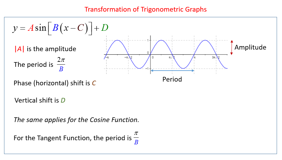
The last thing we need to break down farther is the midline of the function. When you think of midline, think about the maximum and minimum values. The midline is going to be the middle of those values. In this example, the maximum value is 1 and the minimum value is -1. Therefore, the midline of the graph is y=0.
Click the link to continue to the Teacher Discussion.
